Getting started with HubbellGLM: the Barro Colorado Island dataset

Introduction

The HubbellGLM package implements Hubbell regression, a generalized linear model (GLM) for $\alpha$ -diversity (Zito et al. 2026). The model links environmental covariates to Hubbell’s fundamental biodiversity number $\alpha$ , a single dimension-free parameter that controls the rate at which new species accumulate as a function of sample size, and can be converted analytically into Shannon entropy, the Simpson index, and Hill numbers. This bypassess the need to choose which biodiversity index to use in the analysis.

This vignette introduces the statistical framework and demonstrates the package using the Barro Colorado Island (BCI) dataset, a classic tree-census dataset from a 50-ha tropical forest plot in Panama. The original version of the data is downloaded from the R package vegan (Oksanen et al. 2024).

Model details

Hubbell’s fundamental biodiversity number

Let $Y^{(n)}$ denote the number of distinct species (richness) observed in a sample of $n$ individuals drawn from a community. Under Hubbell’s neutral theory of biodiversity (Hubbell 2001), the distribution of $Y^{(n)}$ is given by

$\mathbb{P}(Y^{(n)} = y;\, \alpha) = \frac{\alpha^y \,\Gamma(\alpha)}{\Gamma(\alpha + n)}\,|s(n, y)|, \qquad y = 1, \ldots, n,$

where $|s(n, y)|$ are the (unsigned) Stirling numbers of the first kind, $\Gamma(\cdot)$ is the gamma function, and $\alpha > 0$ is the fundamental biodiversity number (Hubbell 2001). This distribution arises from the Ewens sampling formula (Ewens 1972), which is mathematically equivalent to the Dirichlet process described in (Ferguson 1973) and (Antoniak 1974).

In this model, the richness $Y^{(n)}$ accumulates logarithmically as a function of $n$ , so that $\lim_{n \to \infty} \frac{Y^{(n)}}{\log n} = \alpha.$ This relationship makes $\alpha$ equivalent to the biodiveristy number in the log-series model proposed by (Fisher et al. 1943). A larger $\alpha$ means richer, more even communities; a smaller $\alpha$ means communities dominated by a few abundant species. In particular, the expected species richness in a sample of size $n$ is

$\mu = \mathbb{E}(Y^{(n)}) = \sum_{j=0}^{n-1} \frac{\alpha}{\alpha + j}.$

Hence, the above mean is interpreted as a species accumulation curve that grows logarithmically with $n$ . Moreover, since Hubbell’s model is equivalent to the Dirichlet process, all standard biodiversity indices have closed-form model-based expressions in terms of $\alpha$ (Rigon et al. 2025; Pitman 2006):

Index	Sample-based	Model-based
$\alpha$ -diversity	$\hat\alpha_F \log(1 + n/\hat\alpha_F) = y$	$y = \sum_{j=0}^{n-1} \tfrac{\alpha}{\alpha+j}$
Shannon	$-\sum_k p_k \log p_k$	$\psi(\alpha+1) - \psi(1)$
Simpson	$\sum_k p_k^2$	$1/(\alpha+1)$
Hill ( $q$ )	$\tfrac{1}{q-1}(1 - \sum_k p_k^q)$	$\alpha B(\alpha, q)$

Here $\psi(\cdot)$ is the digamma function, $B(\cdot,\cdot)$ is the beta function, and $p_k$ is the relative abundance of the $k$ -th species.

The Hubbell regression

Since the distribution of $Y^{(n)}$ is an exponential family, we can use it to build a generalized linear model. In particular, our goal is to link the fundamental biodiversity number $\alpha$ with $\mathbf{x} \in \mathbb{R}^p$ . We call this model Hubbell regression. Specifically, letting $i = 1, \ldots, N$ denote the sampling sites (i.e. the observations), we let

$Y_i^{(n_i)} \sim \text{Hubbell}(\alpha_i, n_i), \qquad \log \alpha_i = \eta_i = \mathbf{x}_i^\top \boldsymbol{\beta}.$

This is the canonical link ( $\sigma = 0$ ). A one-unit increase in covariate $x_{ip}$ translates into a $100\%(e^{\beta_p} - 1)$ change in $\alpha$ -diversity.

The polynomial link function

The canonical link constrains species richness to grow logarithmically with $n$ . To allow for heavier-tailed abundance distributions (e.g. arthropods), the package supports a more general polynomial link controlled by $\sigma < 1$ :

$\mu_i = \sum_{j=0}^{n_i - 1} \frac{e^{\eta_i}}{e^{\eta_i} + j^{1-\sigma}}, \qquad \sigma < 1.$

$\sigma = 0$ : logarithmic growth (canonical Hubbell link).
$\sigma \in (0, 1)$ : polynomial growth; the regression-based diversity index is $S_\sigma(\eta) = e^\eta / \sigma$ .
$\sigma < 0$ : finite asymptotic richness.

The parameter $\sigma$ is estimated by maximum likelihood via estimate_sigma() and then held fixed across nested model specifications to ensure comparable regression coefficients.

Robust standard errors: Jaccard-adjusted variance–covariance

Standard GLM inference assumes conditionally independent observations. In species-richness data, the same species may appear in multiple sites, inducing cross-site dependence that the likelihood ignores. HubbellGLM corrects for this using heteroskedastic-consistent sandwich standard errors, where spatial dependence between sites $i$ and $k$ is measured by the Jaccard similarity index $s_{ik}$ (the fraction of shared species between the two samples).

Let $\mathbf{X} \in \mathbb{R}^{N \times p}$ be the design matrix, $\hat{\mathbf{W}} = \text{diag}(\hat{w}_1, \ldots, \hat{w}_N)$ the matrix of IRLS working weights, and $\hat{\mathbf{u}}_i = \partial \log \mathcal{L}(\boldsymbol{\beta}) / \partial \boldsymbol{\beta}|_{\hat{\boldsymbol{\beta}}}$ the score for observation $i$ . The Jaccard-adjusted variance–covariance matrix is

$\widehat{\text{se}}(\hat{\boldsymbol{\beta}}) = (\mathbf{X}^\top \hat{\mathbf{W}} \mathbf{X})^{-1} \left(\sum_{i,k} s_{ik}\, \hat{\mathbf{u}}_i \hat{\mathbf{u}}_k^\top \right) (\mathbf{X}^\top \hat{\mathbf{W}} \mathbf{X})^{-1}.$

This is computed by vcov_species(fit, Dshared), where Dshared is an $N \times N$ matrix of pairwise Jaccard similarities. When species membership between sites is unavailable (as in the BCI example below), the standard Fisher-information-based vcov(fit) is used.

Package functions

`HubbellGLM()` — fit a Hubbell regression

The main fitting function mirrors the syntax of stats::glm. The response is cbind(n, y), where n is the sample size (number of individuals) and y is the observed richness.

fit <- HubbellGLM(cbind(n, y) ~ x1 + x2,
                  family = hubbell(sigma = 0),
                  data   = mydata)

Key arguments:

Argument	Description
`formula`	As in `glm`. Response must be `cbind(n, y)`.
`family`	A Hubbell family object from `hubbell()` or `quasihubbell()`.
`data`	A data frame.

The function returns an object of class HubbellGLM that is compatible with summary(), coef(), vcov(), predict(), residuals(), deviance(), AIC(), BIC(), and step().

`hubbell()` — family object

hubbell(link = "polyseries", sigma = 0)

Sets the GLM family. sigma = 0 gives the canonical (logarithmic) link; any value in $(-\infty, 1)$ gives the polynomial link. Use quasihubbell() for quasi-likelihood inference when the variance is suspected to be inflated.

`estimate_sigma()` — estimate the growth-rate parameter

sigma_hat <- estimate_sigma(cbind(n, y) ~ 1, data = mydata)

Finds the maximum-likelihood $\hat\sigma$ by minimising the BIC of the null model over $\sigma \in (-\infty, 0.9)$ using nlminb. Fix $\sigma$ to this value for all subsequent models to ensure comparability of regression coefficients across nested specifications.

`predict.HubbellGLM()` — predict richness at new sites

predict(fit, newdata = new_sites, type = "response")

type = "link" returns $\hat\eta = \mathbf{x}^\top \hat{\boldsymbol{\beta}}$ .
type = "response" returns the predicted mean richness $\hat\mu = g^{-1}(\hat\eta)$ .

`predict_curve()` — predicted accumulation curve

curve <- predict_curve(fit, xnew = new_site, n = 2000, npoints = 200)

Returns a data frame with columns n (sample size grid), pred (predicted richness), and se (standard error via the delta method). Useful for visualising how richness accumulates at a specific new location.

`vcov_species()` — Jaccard-adjusted variance–covariance

Dshared  <- get_shared_species(species_matrix)  # N x N Jaccard matrix
vcov_adj <- vcov_species(fit, Dshared)

Returns the sandwich variance–covariance matrix described in Section 3. Pass it to lmtest::coeftest(fit, vcov = vcov_adj) to obtain robust z-scores and p-values.

BCI example

The data

The BarroColorado dataset contains 50 subplots from the Barro Colorado Island 50-ha plot. Each row is one subplot with:

n: number of individual trees sampled.
y: number of distinct species observed.
EnvHet: environmental heterogeneity (continuous).
Habitat: habitat type (factor with 5 levels).
Stream: proximity to a stream (Yes/No).

library(HubbellGLM)

data("BarroColorado")
head(BarroColorado)
#>     n   y EnvHet  Habitat Stream
#> 1 448  93 0.6272 OldSlope    Yes
#> 2 435  84 0.3936   OldLow    Yes
#> 3 463  90 0.0000   OldLow     No
#> 4 508  94 0.0000   OldLow     No
#> 5 505 101 0.4608 OldSlope     No
#> 6 412  85 0.0768   OldLow     No

plot(BarroColorado$n, BarroColorado$y,
     col  = as.integer(BarroColorado$Habitat),
     pch  = 16, cex = 0.9,
     xlab = "Sample size (n)",
     ylab = "Observed richness (y)",
     main = "BCI: richness vs. sample size")
legend("bottomright", legend = levels(BarroColorado$Habitat),
       col = 1:5, pch = 16, cex = 0.8)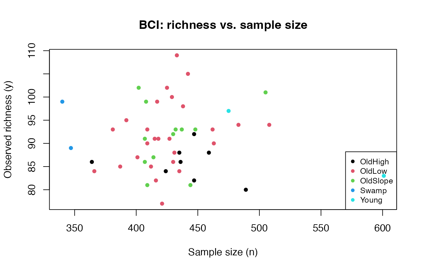

Observed species accumulation: richness vs. sample size across habitat types.

The canonical link (logarithmic growth)

These are three models run with the canonical link

# M0: the null model
fit_null <- HubbellGLM(cbind(n, y) ~ 1,
                     family = hubbell(sigma = 0),
                     data   = BarroColorado)

# M1: environmental heterogeneity only
fit_M1 <- HubbellGLM(cbind(n, y) ~ EnvHet,
                     family = hubbell(sigma = 0),
                     data   = BarroColorado)

# M2: add habitat type
fit_M2 <- HubbellGLM(cbind(n, y) ~ EnvHet + Habitat,
                     family = hubbell(sigma = 0),
                     data   = BarroColorado)

# M3: add stream proximity
fit_M3 <- HubbellGLM(cbind(n, y) ~ EnvHet + Habitat + Stream,
                     family = hubbell(sigma = 0),
                     data   = BarroColorado)

summary(fit_M3)
#> 
#> Call:
#> HubbellGLM(formula = cbind(n, y) ~ EnvHet + Habitat + Stream, 
#>     family = hubbell(sigma = 0), data = BarroColorado)
#> 
#> Coefficients:
#>                 Estimate Std. Error z value Pr(>|z|)    
#> (Intercept)      3.43326    0.05523  62.161  < 2e-16 ***
#> EnvHet           0.07146    0.09230   0.774  0.43880    
#> HabitatOldLow    0.14270    0.05534   2.579  0.00992 ** 
#> HabitatOldSlope  0.13352    0.06224   2.145  0.03193 *  
#> HabitatSwamp     0.26655    0.11023   2.418  0.01560 *  
#> HabitatYoung    -0.04071    0.10360  -0.393  0.69439    
#> StreamYes       -0.10782    0.05879  -1.834  0.06665 .  
#> ---
#> Signif. codes:  0 '***' 0.001 '**' 0.01 '*' 0.05 '.' 0.1 ' ' 1
#> 
#> (Dispersion parameter for hubbell family taken to be 1)
#> 
#>     Null deviance: 49.331  on 49  degrees of freedom
#> Residual deviance: 34.543  on 43  degrees of freedom
#> AIC: 343.26
#> 
#> Number of Fisher Scoring iterations: 3

Interpreting coefficients

Coefficients are on the log- $\alpha$ scale. A coefficient $\hat\beta_p$ means a one-unit increase in $x_p$ is associated with a $100\%(e^{\hat\beta_p} - 1)$ change in $\alpha$ -diversity.

round(100 * (exp(coef(fit_M3)) - 1), 2)
#>     (Intercept)          EnvHet   HabitatOldLow HabitatOldSlope    HabitatSwamp 
#>         2997.75            7.41           15.34           14.28           30.55 
#>    HabitatYoung       StreamYes 
#>           -3.99          -10.22

Model comparison via deviance

cat("Null deviance:    ", round(deviance(fit_null), 1), "\n")
#> Null deviance:     49.3
cat("M1 deviance:      ", round(deviance(fit_M1),  1), "\n")
#> M1 deviance:       49.2
cat("M2 deviance:      ", round(deviance(fit_M2),  1), "\n")
#> M2 deviance:       37.9
cat("M3 deviance:      ", round(deviance(fit_M3),  1), "\n")
#> M3 deviance:       34.5

The pseudo- $R^2$ for each model relative to the null:

1 - deviance(fit_M3) / deviance(fit_null)
#> [1] 0.2997722

Predicted accumulation curves

predict_curve() returns the fitted accumulation curve (with pointwise standard errors) at any new covariate combination. Here we compare a high-heterogeneity OldHigh subplot with a near-stream Young subplot.

new_sites <- data.frame(
  n       = c(500, 500),
  y       = c(1L,  1L),      # placeholder required by the formula
  EnvHet  = c(0.6,  0.0),
  Habitat = factor(c("OldHigh", "OldSlope"),
                   levels = levels(BarroColorado$Habitat)),
  Stream  = factor(c("No", "Yes"),
                   levels = levels(BarroColorado$Stream))
)

curve1 <- predict_curve(fit_M3, xnew = new_sites[1, ], n = 600, npoints = 100)
curve2 <- predict_curve(fit_M3, xnew = new_sites[2, ], n = 600, npoints = 100)

pred1 <- curve1$mean[, 1]; se1 <- curve1$se[, 1]
pred2 <- curve2$mean[, 1]; se2 <- curve2$se[, 1]

plot(curve1$n, pred1, type = "l", col = "steelblue", lwd = 2,
     ylim = range(c(pred1 - 2*se1, pred2 + 2*se2)),
     xlab = "Sample size (n)", ylab = "Predicted richness",
     main = "Predicted accumulation curves")
lines(curve2$n, pred2, col = "tomato", lwd = 2)

# 95% CI bands
polygon(c(curve1$n, rev(curve1$n)),
        c(pred1 - 2*se1, rev(pred1 + 2*se1)),
        col = adjustcolor("steelblue", 0.15), border = NA)
polygon(c(curve2$n, rev(curve2$n)),
        c(pred2 - 2*se2, rev(pred2 + 2*se2)),
        col = adjustcolor("tomato", 0.15), border = NA)

legend("bottomright",
       legend = c("OldHigh, high EnvHet, no stream",
                  "Young, low EnvHet, near stream (OldSlope fixed)"),
       col = c("steelblue", "tomato"), lwd = 2, cex = 0.8)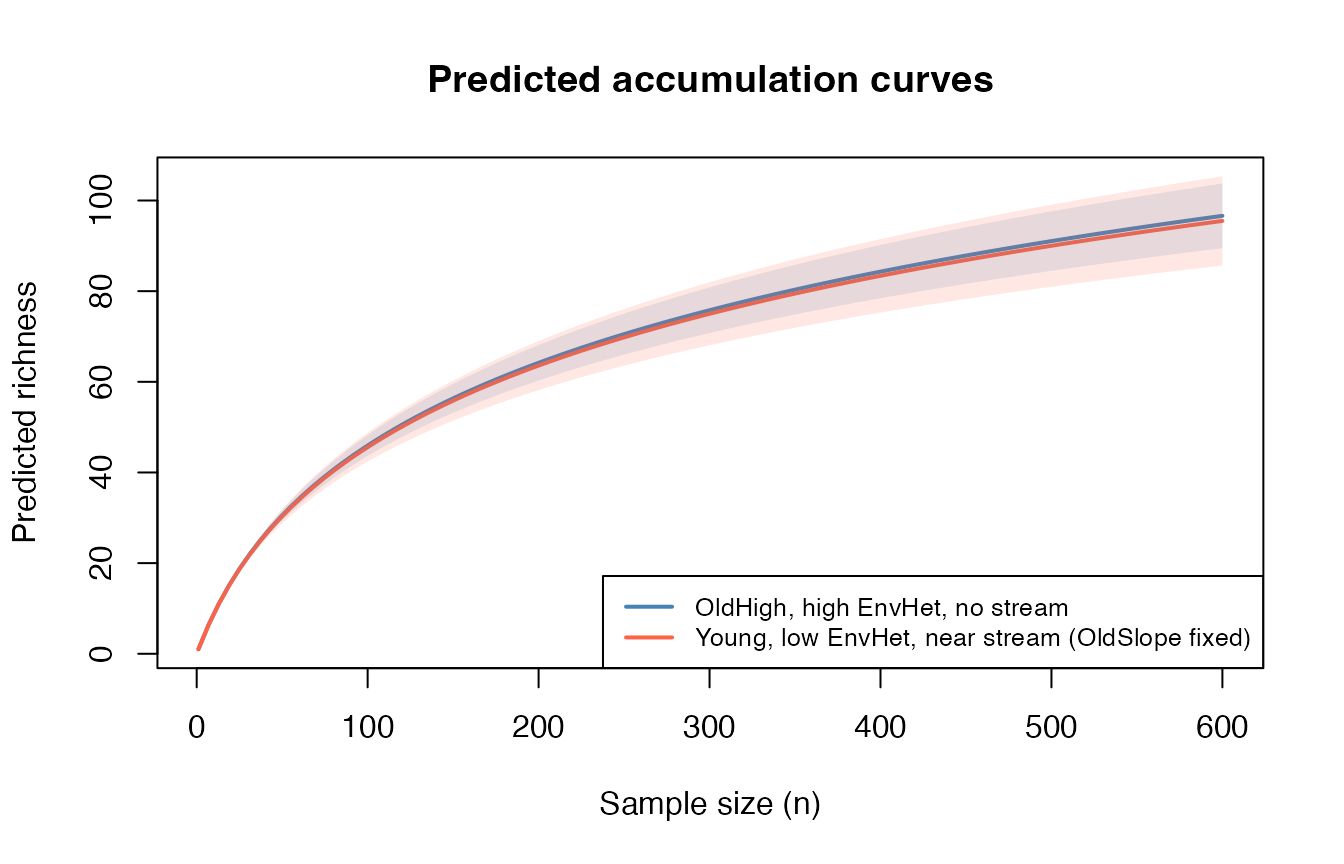

Predicted accumulation curves for two contrasting subplot types.

Derived biodiversity indices

Once $\hat\alpha$ is recovered from the fitted model, all standard biodiversity indices follow analytically.

alpha_n <- function(mu, n) {
  uniroot(function(a) mean_dirichlet_process(a, n) - mu,
          c(1e-6, 1e6))$root
}

# Predictions at n = 500 for each subplot
mu_pred <- predict(fit_M3, type = "response")
n_vec   <- BarroColorado$n

alpha_vals   <- mapply(alpha_n, mu_pred, n_vec)
shannon_vals <- digamma(alpha_vals + 1) - digamma(1)
simpson_vals <- 1 / (alpha_vals + 1)

cat("Median alpha:   ", round(median(alpha_vals),   3), "\n")
#> Median alpha:    35.729
cat("Median Shannon: ", round(median(shannon_vals), 3), "\n")
#> Median Shannon:  4.167
cat("Median Simpson: ", round(median(simpson_vals), 4), "\n")
#> Median Simpson:  0.0272

Model comparison via AIC and BIC

Compare nested models directly using AIC() and BIC().

aic_vals <- c(
  Null     = AIC(fit_null),
  EnvHet   = AIC(fit_M1),
  `+Habitat` = AIC(fit_M2),
  `+Stream`  = AIC(fit_M3)
)
bic_vals <- c(
  Null     = BIC(fit_null),
  EnvHet   = BIC(fit_M1),
  `+Habitat` = BIC(fit_M2),
  `+Stream`  = BIC(fit_M3)
)
round(rbind(AIC = aic_vals, BIC = bic_vals), 2)
#>       Null EnvHet +Habitat +Stream
#> AIC 346.05 347.89   344.66  343.26
#> BIC 347.96 351.71   356.13  356.65

The model with the lowest AIC/BIC is preferred. Note that step.HubbellGLM() can also be called directly for automated backward/forward selection; see ?step.hubbell.

Estimate $\sigma$

Before fitting any covariate model, estimate the accumulation-curve growth rate from the null model.

sigma_hat <- estimate_sigma(formula = fit_M3$formula, data = BarroColorado)
#> Evaluating sigma =  0 
#> Evaluating sigma =  1.490116e-08 
#> Evaluating sigma =  -1 
#> Evaluating sigma =  -0.9999822 
#> Evaluating sigma =  -0.9063331 
#> Evaluating sigma =  -0.90634 
#> Evaluating sigma =  -0.2472168 
#> Evaluating sigma =  -0.7269597 
#> Evaluating sigma =  -0.7269794 
#> Evaluating sigma =  -0.5742515 
#> Evaluating sigma =  -0.5742655 
#> Evaluating sigma =  -0.6462702 
#> Evaluating sigma =  -0.6462601 
#> Evaluating sigma =  -0.6373282 
#> Evaluating sigma =  -0.6373377 
#> Evaluating sigma =  -0.6373282
cat("Estimated sigma:", round(sigma_hat, 4), "\n")
#> Estimated sigma: -0.6373

A value near zero indicates near-logarithmic growth, which is consistent with the Dirichlet-process baseline. Values in $(0, 1)$ indicate polynomial (heavier-tailed) growth, while $\sigma < 0$ implies that the accumulation curve eventually converges to a finite number. —

Session information

sessionInfo()
#> R version 4.6.0 (2026-04-24)
#> Platform: aarch64-apple-darwin23
#> Running under: macOS Tahoe 26.5.1
#> 
#> Matrix products: default
#> BLAS:   /Library/Frameworks/R.framework/Versions/4.6/Resources/lib/libRblas.0.dylib 
#> LAPACK: /Library/Frameworks/R.framework/Versions/4.6/Resources/lib/libRlapack.dylib;  LAPACK version 3.12.1
#> 
#> locale:
#> [1] en_CA.UTF-8/en_CA.UTF-8/en_CA.UTF-8/C/en_CA.UTF-8/en_CA.UTF-8
#> 
#> time zone: America/Toronto
#> tzcode source: internal
#> 
#> attached base packages:
#> [1] stats     graphics  grDevices utils     datasets  methods   base     
#> 
#> other attached packages:
#> [1] HubbellGLM_1.0.0
#> 
#> loaded via a namespace (and not attached):
#>  [1] cli_3.6.6         knitr_1.51        rlang_1.2.0       xfun_0.58        
#>  [5] otel_0.2.0        textshaping_1.0.5 jsonlite_2.0.0    htmltools_0.5.9  
#>  [9] ragg_1.5.2        sass_0.4.10       stats4_4.6.0      rmarkdown_2.31   
#> [13] evaluate_1.0.5    jquerylib_0.1.4   fastmap_1.2.0     yaml_2.3.12      
#> [17] lifecycle_1.0.5   compiler_4.6.0    codetools_0.2-20  fs_2.1.0         
#> [21] Rcpp_1.1.1-1.1    systemfonts_1.3.2 digest_0.6.39     R6_2.6.1         
#> [25] bslib_0.11.0      tools_4.6.0       pkgdown_2.2.0     cachem_1.1.0     
#> [29] desc_1.4.3

References

Antoniak, Charles E. 1974. “Mixtures of Dirichlet Processes with Applications to Bayesian Nonparametric Problems.” The Annals of Statistics 2 (6): 1152–74.

Ewens, Warren J. 1972. “The Sampling Theory of Selectively Neutral Alleles.” Theoretical Population Biology 3 (1): 87–112.

Ferguson, Thomas S. 1973. “A Bayesian Analysis of Some Nonparametric Problems.” The Annals of Statistics 1 (2): 209–30.

Fisher, Ronald A., A. Steven Corbet, and C. B. Williams. 1943. “The Relation Between the Number of Species and the Number of Individuals in a Random Sample of an Animal Population.” Journal of Animal Ecology 12 (1): 42–58.

Hubbell, Stephen P. 2001. The Unified Neutral Theory of Biodiversity and Biogeography. Princeton University Press.

Oksanen, Jari, Gavin L. Simpson, F. Guillaume Blanchet, et al. 2024. Vegan: Community Ecology Package. https://CRAN.R-project.org/package=vegan.

Pitman, Jim. 2006. Combinatorial Stochastic Processes. Vol. 1875. Lecture Notes in Mathematics. Springer.

Rigon, Tommaso, Cheng-Long Hsu, and David B. Dunson. 2025. “A Bayesian Theory for Estimation of Biodiversity.” arXiv:2502.01333.

Zito, Alessandro, Tommaso Rigon, Tomas Roslin, et al. 2026. “Predicting Global Biodiversity via Hubbell Regression.” BioArxiv.

Alessandro Zito